Ariel's Commute

How long does Ariel's commute take, and does it matter when she leaves?
Ariel grabbed her data from Moves. Here I'm going to see how time-of-day affects her commute duration.
Side note: Kudos to Moves for excellent export facilities. Absolutely wonderful. They give you the data in every format and breakdown imaginable.
%pylab inline
import pandas as pd
import seaborn
df = pd.read_csv('storyline.csv')
df['Start'] = pd.to_datetime(df['Start'])
# we only want since the current commute started
df = df[df['Start'] > '2015-03-01']
df.head()
| Date | Type | Name | Start | End | Duration | |
|---|---|---|---|---|---|---|
| 4897 | 3/1/15 | place | Home | 2015-03-01 05:00:00 | 2015-03-01T11:17:27-05:00 | 40647 |
| 4898 | 3/1/15 | move | transport | 2015-03-01 16:17:27 | 2015-03-01T11:49:20-05:00 | 1913 |
| 4899 | 3/1/15 | move | walking | 2015-03-01 16:49:19 | 2015-03-01T11:56:58-05:00 | 459 |
| 4900 | 3/1/15 | place | Place in Cambridgeport | 2015-03-01 16:56:59 | 2015-03-01T14:12:03-05:00 | 8104 |
| 4901 | 3/1/15 | move | walking | 2015-03-01 19:12:03 | 2015-03-01T14:19:04-05:00 | 421 |
Later I'm going to only want the time of day, not the date, so set all dates to 1970-01-01.
df['Start'] = df['Start'].apply(lambda x: x.replace(year=1970, month=1, day=1))
I want to know which transport rows go between Home and Koch, so I make two new columns shifting name up and down so I can match against those.
df['prev_name'] = df['Name'].shift(1)
df['next_name'] = df['Name'].shift(-1)
df.head()
| Date | Type | Name | Start | End | Duration | prev_name | next_name | |
|---|---|---|---|---|---|---|---|---|
| 4897 | 3/1/15 | place | Home | 1970-01-01 05:00:00 | 2015-03-01T11:17:27-05:00 | 40647 | NaN | transport |
| 4898 | 3/1/15 | move | transport | 1970-01-01 16:17:27 | 2015-03-01T11:49:20-05:00 | 1913 | Home | walking |
| 4899 | 3/1/15 | move | walking | 1970-01-01 16:49:19 | 2015-03-01T11:56:58-05:00 | 459 | transport | Place in Cambridgeport |
| 4900 | 3/1/15 | place | Place in Cambridgeport | 1970-01-01 16:56:59 | 2015-03-01T14:12:03-05:00 | 8104 | walking | walking |
| 4901 | 3/1/15 | move | walking | 1970-01-01 19:12:03 | 2015-03-01T14:19:04-05:00 | 421 | Place in Cambridgeport | transport |
koch = 'MIT Koch Day Care Ctr'
east = df.loc[(df.Name == 'transport') & (df.prev_name == 'Home') & (df.next_name == koch) ]
west = df.loc[(df.Name == 'transport') & (df.next_name == 'Home') & (df.prev_name == koch) ]
east.head()
| Date | Type | Name | Start | End | Duration | prev_name | next_name | |
|---|---|---|---|---|---|---|---|---|
| 4945 | 3/5/15 | move | transport | 1970-01-01 12:49:44 | 2015-03-05T08:45:36-05:00 | 3352 | Home | MIT Koch Day Care Ctr |
| 4983 | 3/9/15 | move | transport | 1970-01-01 11:50:58 | 2015-03-09T08:32:02-04:00 | 2464 | Home | MIT Koch Day Care Ctr |
| 5059 | 3/16/15 | move | transport | 1970-01-01 12:03:33 | 2015-03-16T08:40:40-04:00 | 2227 | Home | MIT Koch Day Care Ctr |
| 5075 | 3/17/15 | move | transport | 1970-01-01 12:16:17 | 2015-03-17T08:49:58-04:00 | 2021 | Home | MIT Koch Day Care Ctr |
| 5093 | 3/18/15 | move | transport | 1970-01-01 12:21:08 | 2015-03-18T08:51:00-04:00 | 1792 | Home | MIT Koch Day Care Ctr |
plot(west.Start,west.Duration,'.') # not bothering to make the x axis a date for now
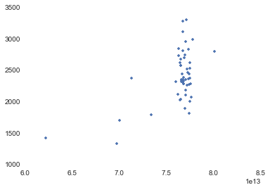
Let's get rid of outliers.
Yes, obviously if you leave work in the middle of the day, there's zero traffic, but we don't want those 5 points driving the entire model, so let's drop them.
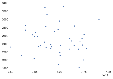
west = west.ix[(west.Start > 7.5e13) & (west.Start < 8e13)].copy()
plot(west.Start,west.Duration,'.')
plot(east.Start,east.Duration,'.')
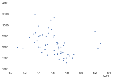
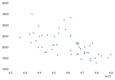
east = east.ix[(east.Start > 4.2e13) & (east.Start < 5e13)].copy()
plot(east.Start,east.Duration,'.')
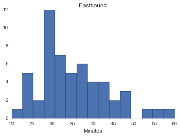
How long does the commute take?
hist([k/60 for k in east.Duration], 15, [20, 60])
# using pyplot.hist instead of DataFrame.hist so I can /60 to get minutes
title('Eastbound')
xlabel('Minutes')
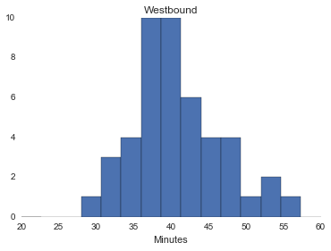
hist([k/60 for k in west.Duration], 15, [20, 60])
title('Westbound')
xlabel('Minutes')
Write to file.
east.to_csv('east.csv')
west.to_csv('west.csv')
Now, do some statistics, in R
Thanks to @ozjimbob for most of this.
Load in the data and convert the times to a POSIXct class, then make them numeric because gam models don’t always play nice with this class. So we have seconds from the UNIX epoch.
I'm also going to convert Duration to minutes, because who thinks in seconds.
east=read.csv("east.csv", stringsAsFactors=FALSE)
west=read.csv("west.csv" , stringsAsFactors=FALSE)
east$Start=as.numeric(as.POSIXct(east$Start))
west$Start=as.numeric(as.POSIXct(west$Start))
east$Start = east$Start - 3600*4   # fix time zones back to US/Eastern
west$Start = west$Start - 3600*4
east$Duration = east$Duration / 60
west$Duration = west$Duration / 60
We’re going to do generalized additive models that allow you to fit a spline smooth through a predictor variable.
e_mod=mgcv::gam(Duration ~ s(Start),data=east)
w_mod=mgcv::gam(Duration ~ s(Start),data=west)
Let's examine the summaries for these.
East
summary(e_mod)
##
## Family: gaussian
## Link function: identity
##
## Formula:
## Duration ~ s(Start)
##
## Parametric coefficients:
##             Estimate Std. Error t value Pr(>|t|)
## (Intercept)  35.4346     0.8483   41.77   <2e-16 ***
## ---
## Signif. codes:  0 '***' 0.001 '**' 0.01 '*' 0.05 '.' 0.1 ' ' 1
##
## Approximate significance of smooth terms:
##            edf Ref.df     F  p-value
## s(Start) 6.574  7.712 6.318 1.18e-05 ***
## ---
## Signif. codes:  0 '***' 0.001 '**' 0.01 '*' 0.05 '.' 0.1 ' ' 1
##
## R-sq.(adj) =   0.46   Deviance explained = 52.7%
## GCV = 45.195  Scale est. = 38.856    n = 54
West
summary(w_mod)
##
## Family: gaussian
## Link function: identity
##
## Formula:
## Duration ~ s(Start)
##
## Parametric coefficients:
##             Estimate Std. Error t value Pr(>|t|)
## (Intercept)  41.2279     0.8465    48.7   <2e-16 ***
## ---
## Signif. codes:  0 '***' 0.001 '**' 0.01 '*' 0.05 '.' 0.1 ' ' 1
##
## Approximate significance of smooth terms:
##          edf Ref.df     F p-value
## s(Start)   1      1 0.139   0.711
##
## R-sq.(adj) =  -0.0195   Deviance explained = 0.316%
## GCV = 34.463  Scale est. = 32.965    n = 46
West looks terrible - there's just nothing there. Let's start with East.
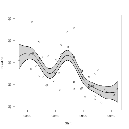
East - morning commute to work
Let’s look at the east model - generate predictions, with standard errors, for each possible time between the minimum and maximum.
pred_frame=data.frame(Start=min(east$Start):max(east$Start))

e_predict=predict(e_mod,newdata = pred_frame,se.fit=TRUE)

pred_frame$pred=e_predict$fit
pred_frame$upper=e_predict$fit + e_predict$se.fit
pred_frame$lower=e_predict$fit - e_predict$se.fit
Now prepare a graph - plot the predicted fit with the error bars. Convert the times back into POSIXct for nice plotting too.
pgoe_x = c(pred_frame$Start,rev(pred_frame$Start))
pgoe_y = c(pred_frame$upper,rev(pred_frame$lower))

pred_frame$Start_po=as.POSIXct(pred_frame$Start,origin="1970-01-01")

plot(pred_frame$pred ~ pred_frame$Start_po,type="l",ylim=c(20,60),xlab="Start",ylab="Duration")
polygon(pgoe_x,pgoe_y,col="#44444444")
points(east$Duration ~ east$Start)
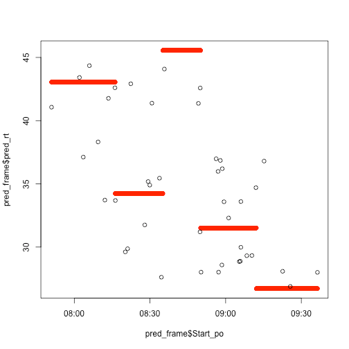
Let's try a regression tree.
rp_mod=rpart(Duration ~ Start,data=east)
rp_predict=predict(rp_mod,newdata=pred_frame)
pred_frame$pred_rt = rp_predict
plot(pred_frame$pred_rt ~ pred_frame$Start_po,col="red")
points(east$Duration ~ east$Start)
And a randomForest.
rf_mod=randomForest(Duration ~ Start,data=east)
print(rf_mod)
##
## Call:
##  randomForest(formula = Duration ~ Start, data = east)
##                Type of random forest: regression
##                      Number of trees: 500
## No. of variables tried at each split: 1
##
##           Mean of squared residuals: 53.52246
##                     % Var explained: 24.24
Plot the model predictions.
rf_predict=predict(rf_mod,newdata=pred_frame,type="response")
pred_frame$pred_rf = rf_predict
plot(pred_frame$pred_rf ~ pred_frame$Start_po,col="red")
points(east$Duration ~ east$Start)
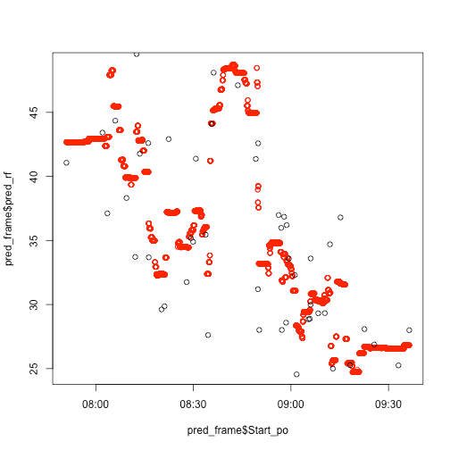
It's insanely overfitted, but ok.
West - evening ride home
Let’s look at the west plot.
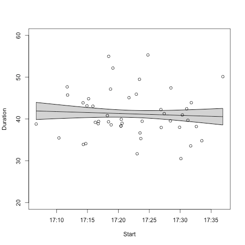
Ariel leaves work in such a narrow window that there's just no difference in the small changes she makes. Maybe in the future she can start experimenting with intentionally leaving later to see what that does to her commute time.
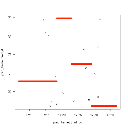
Everything's going to be garbage, but let's look anyway. Regression tree:
randomForest.
print(rf_mod)
##
## Call:
##  randomForest(formula = Duration ~ Start, data = west)
##                Type of random forest: regression
##                      Number of trees: 500
## No. of variables tried at each split: 1
##
##           Mean of squared residuals: 49.80263
##                     % Var explained: -57.45
lol negative variance
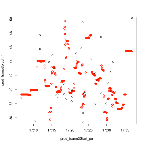
lol nope